Application to breast cancer dataset#

Prepare dataset#

Load#

import numpy as np
import pandas as pd

pd.options.display.max_columns = 10

from sklearn.model_selection import train_test_split
from sklearn.datasets import load_breast_cancer

data = load_breast_cancer()
data_X, data_y = data.data, data.target

X = pd.DataFrame(data=data_X, columns=data.feature_names)
y = pd.Series(data_y)

Create artificial categorical variable#

For illustration purposes, create a random categorical feature

X["category"] = np.where(X["mean smoothness"] <= 0.1, "A", "B")

Split train/test#

X_train, X_test, y_train, y_test = train_test_split(
    X, y, test_size=0.25, random_state=0
)

Create unknown category in test set#

To illustrate robustness of implementation, create unknown category in test set

X_test["category"] = "C"

Automatically create binary features#

Call EBMBinarizer#

The binary feature creation is based on train dataset.
The train and test dataset are then transformed for training and evaluation.

from scorepyo.binarizers import EBMBinarizer


binarizer = EBMBinarizer(max_number_binaries_by_features=3, keep_negative=True)
binarizer.fit(X_train, y_train, categorical_features="auto", to_exclude_features=None)

X_train_binarized = binarizer.transform(X_train)
X_test_binarized = binarizer.transform(X_test)

X_train_binarized.sample(3)

	mean radius < 12.26	12.26 <= mean radius < 14.66	mean radius >= 14.66	mean texture < 17.2	17.2 <= mean texture < 20.66	...	0.07 <= worst fractal dimension < 0.09	category_A
401	0	1	0	0	0	...	1	1
5	1	0	0	0	1	...	1	1
316	0	0	1	1	0	...	1	1

3 rows × 92 columns

Display information from binarizer#

The binarizer also computes a dataframe containing information about the binarizing process. This information is later used to for the risk-score model.

It contains the following information for each binary feature created:

name of binary feature
log-odd coefficient of the binary feature according to EBM underlying model
lower and upper threshold value used for creating the interval on the original feature domain
category value if the original feature was categorical
original feature name
original feature type
number of samples with a positive value on this binary feature
name of the original feature

binarizer.get_info()

	log_odds	lower_threshold	upper_threshold	category_value	feature	type	density
binary_feature
mean radius < 12.26	0.135708	NaN	12.26	None	mean radius	continuous	142
12.26 <= mean radius < 14.66	0.086529	12.26	14.66	None	mean radius	continuous	142
mean radius >= 14.66	-0.222237	14.66	NaN	None	mean radius	continuous	142
mean texture < 17.2	0.740917	NaN	17.205	None	mean texture	continuous	142
17.2 <= mean texture < 20.66	0.056726	17.205	20.665	None	mean texture	continuous	142
...	...	...	...	...	...	...	...
0.07 <= worst fractal dimension < 0.09	0.372596	0.07428	0.08649	None	worst fractal dimension	continuous	142
worst fractal dimension >= 0.09	-0.156302	0.08649	NaN	None	worst fractal dimension	continuous	142
category_A	0.192341	None	None	A	category	categorical	266
category_B	-0.319767	None	None	B	category	categorical	160
intercept	1.367172	None	None	None	intercept	None	None

93 rows × 7 columns

Train RiskScore model#

The RiskScore models can take several parameters divided into three sets:

Binarizer parameter :
- binarizer: binarizer to use for the risk score model
Risk score cards parameters : defines the property of the score card
- nb_max_features: number of maximum binary features to use for the risk score model
- min_point_value: minimum possible number of points for each binary feature
- max_point_value: maximum possible number of points for each binary feature
Exploration/fitting parameters : defines the different exploration phase of the risk score model
- ranker: ranker of binary features
- nb_additional_features: number of additional features to take into the subset of binary features according to the ranker
- enumeration_maximization_metric: maximization metric that will be used to elicit the best enumerated combination
- calibrator: calibrator of probabilities for each score

EBMRiskScore is a child class of RiskScore, that automatically uses EBMBinarizer as a binarizer.

from scorepyo.models import EBMRiskScore


scorepyo_model = EBMRiskScore(
    nb_max_features=4,
    min_point_value=-1,
    max_point_value=2,
)

scorepyo_model.fit(X_train, y_train)

<scorepyo.models.EBMRiskScore at 0x1f8437cdc40>

Display the summary of the risk score model#

The summary of the risk score built by the model.

It displays two elements :

Feature-point card : Points for each selected binary feature
Score card : Scores (=sum of points) with their associated probability

scorepyo_model.summary()

======================
| FEATURE-POINT CARD |
======================
| Feature              | Description                  | Point(s)   |       |
|:---------------------|:-----------------------------|:-----------|:------|
| worst concave points | worst concave points >= 0.14 | -1         | ...   |
| area error           | area error >= 33.35          | -1         | + ... |
| worst radius         | worst radius >= 16.66        | -1         | + ... |
| worst texture        | worst texture < 22.66        | 1          | + ... |
|                      |                              | SCORE=     | ...   |

=======================================
=======================================

======================
|     SCORE CARD     |
======================
| SCORE   | -3    | -2    | -1     | 0      | 1      |
|:--------|:------|:------|:-------|:-------|:-------|
| RISK    | 0.00% | 2.50% | 46.15% | 95.83% | 99.10% |

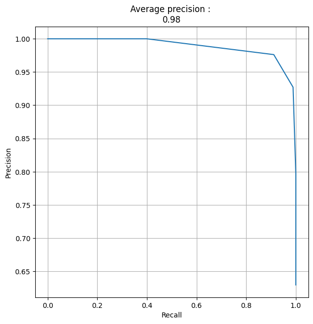
Evaluation on test set#

Precision-Recall curve on test set#

import matplotlib.pyplot as plt
from sklearn.metrics import precision_recall_curve, average_precision_score


y_proba = scorepyo_model.predict_proba(X_test)[:, 1].reshape(-1, 1)

precision, recall, thresholds = precision_recall_curve(y_test.astype(int), y_proba)
fig, ax = plt.subplots(figsize=(7, 7))
plt.plot(recall, precision)
average_precision = np.round(average_precision_score(y_test.astype(int), y_proba), 3)
title_PR_curve = f"Average precision : \n{average_precision}"
plt.title(title_PR_curve)
plt.xlabel("Recall")
plt.ylabel("Precision")
plt.grid()
plt.show()

Application to breast cancer dataset

Contents